Timing Archives – Page 2 of 2 – The Broadcast Knowledge

Good timing is essential in production for AES67 audio and SMPTE ST 2110. Delivering timing is no longer a matter of delivering a signal throughout your facility, over IP timing is bidirectional and forms a system which should be monitored and managed. Timing distribution has always needed design and architecture, but the detail and understanding needed are much more. At the beginning of this talk, Andreas Hildebrand explains why we need to bother with such complexity, after all, we got along very well for many years without it! Non-IP timing signals are distributed on their own cables as part of their own system. There are some parts of the chain which can get away without timing signals, but when they are needed, they are on a separate cable. With IP, having a separate network for distribution of timing doesn’t make sense so, whether you have an analogue or digital timing signal, that needs to be moving into the IP domain. But how much accuracy in timing to you need? Network devices already widely use NTP which can achieve an accuracy of less than a millisecond. Andreas explains that this isn’t enough for professional audio. At 48Khz, AES samples happen at an accuracy of plus or minus 10 microseconds with 192KHz going down to 2.5 microseconds. As your timing signal has to be less than the accuracy you need, this means we need to achieve nanosecond precision.

Daniel Boldt from timing specialists Meinberg is the focus of this talk explaining how we achieve this nano-second precision. Enter PTP, the Precision Time Protocol. This is a cross-industry standard from the IEEE uses in telcoms, power, finance and in many others wherever a network and its devices need to understand the time. It’s not a static standard, Daniel explains, and it’s just about to see its third revision which, like the last, adds features.

Before finding out about the latest changes, Daniel explains how PTP works in the first place; how is it possible to accurately derive time down to the nanosecond over a network which will have variable propagation times? We see how timestamps are introduced into the network interface controller (NIC) at the last moment allowing the timestamps to be created in hardware which removes some of the variable delays that is typical in software. This happens, Daniel shows, in the switch as well as in the server network cards. This article will refer to either a primary clock or a grand master. Daniel steps us through the messages exchanged between the primary and secondary clock which is the interaction at the heart of the protocol. The key is that after the primary has sent a timestamp, the secondary sends its timestamp to the primary which replies saying the time it received the secondary the reply. The secondary ends up with 4 timestamps that it can combine to determine its offset from the primary’s time and the delay in receiving messages. Applying this information allows it to correct the clock very accurately.

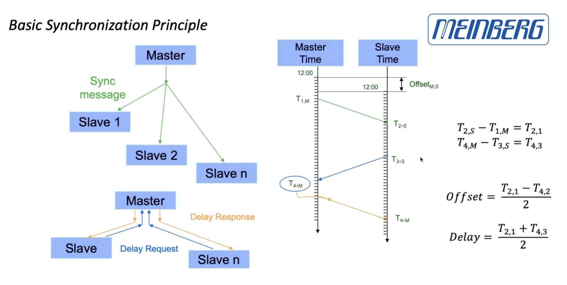
PTP Primary-Secondary Message Exchange.
Source: Meinberg

Most broadcasters would prefer to have more than one grandmaster clock but if there are multiple clocks, how do you choose which to sync from? Timing systems have long used strata whereby clocks are rated based on accuracy, either for internal accuracy & stability or by what they are synched to. This is also true for PTP and is part of the considerations in the ‘Best Master Clock Algorithm’. The BMCA starts by allowing a time source to assess its own accuracy and then search for better options on the network. Clocks announce themselves to the network and by listening to other announcements, a clock can decide if it should become a primary clock if, for instance, it hears no announce messages at all. For devices which should never be a grand primary, you can force them never to decide to become grand masters. This is a requisite for audio devices participating in ST 2110-3x.

Passing PTP around the network takes some care and is most easily done by using switches which understand PTP. These switches either run a ‘boundary clock’ or are ‘transparent clocks’. Daniel explores both of these scenarios explaining how the boundary clock switch is able to run multiple primary and secondary clocks depending on what is connected on each interface. We also see what work the switches have to do behind the scenes to maintain timing precision in transparent mode. In summary, Daniel summaries boundary clocks as being good for hierarchical systems and scales well but requires continuous monitoring whereas transparent clocks are simpler to deploy and require minimal monitoring. The main issue with transparent clocks is that they don’t scale well as all your timing messages are still going back to one main clock which could get overwhelmed.

SMPTE 2022-7 has been a very successful standard as its reliance only on RTP has allowed it to be widely applicable to compressed and uncompressed IP flows. It is often used in 2110 networks, too, where two separate networks are run and brought together at the receiving device. That device, on a packet-by-packet basis, is free to derive its audio/video stream from either network. This requires, however, exactly the same timing on both networks so Daniel looks at an example diagram where this PTP sharing is shown.

PTP’s still evolving and in this next section, Daniel takes us through some of the coming improvements which are also outlined at Meinberg’s blog. These are profile isolation, multi-domain clocks, security improvements and more.

Andreas takes the final section of the webinar to explain how we use PTP in media networks. All receivers will have the same clock which could be derived from GPS removing the need to distribute PTP between sites. 2110 is based on RTP which requires a timestamp to be added to every packet delivered to the network. RTP is a wrapper around IP packets which includes a timestamp which can be derived from the media clock counter.

Andreas looks at how accurate RTP delivery is achieved, dealing with offset values, populating the timestamp from the PTP clock for realties streams and he explains how the playout delay is calculated from the link offset. Finally, he shows the relatively simple process of synchronisation art the playout device. With all the timestamps in the system, synchronising playback of audio, video and metadata using buffers can be achieved fairly easily. Unfortunately, timestamps are easily destroyed by secondary processing (for instance loudness adjustment for an audio stream). Clearly, if this happened, synchronisation at the receiver would be broken. Whilst this will be addressed by out-of-band messaging in future standards, for now, this is managed by a broadcast controller which can take delay information from processing stages and distribute this to receivers.

Watch now!
Speakers

	Daniel Boldt Head of Software Development, Meinberg
	Andreas Hildebrand RAVENNA Technology Evangelist, ALC NetworX

Timing and synchronisation have always been a fundamental aspect of TV and as we move to IP, we see that timing is just as important. Whilst there are digital workflows that don’t need to be synchronised against each other, many do such as studio productions. However, as we see in this talk from The Broadcast Bridge’s Tony Orme, IP networks make timing all the more variable and accounting for this is key to success.

To start with Tony looks at the way the OBs, also known as REMIs, are moving to IP and need a timing plane across all of the different parts of production. We see how traditionally synchronisation is needed and the effect of timing problems not only in missed data but also with all essences being sent separately synchronisation problems between them can easily creep in.

When it comes to IP timing itself, Tony explains how PTP is used to record the capture time of the media/essences and distribute through the system. Looking at the data on the wire and the interval between that and the last will show a distribution of, hopefully, a few microseconds variation. This variation gives rise to jitter which is a varying delay in data arrival. The larger the spread, the more difficult it will be to recover data. To examine this more closely, Tony looks at the reasons for and the impacts of congestion, jitter, reordering of data.

Bursting, to make one of these as an example, is a much overlooked issue on networks. While it can occur in many scenarios without any undue problems, microbusting can be a major issue and one that you need to look for to find. This surrounds the issue of how you decide that a data flow is, say, 500Mbps. If you had an encoder which sent data at 1Gbps for 5 minutes and no data for 5 minutes, then over the 10 minute window, the average bitrate would have been 500Mbps. This clearly isn’t a 500Mbps encoder, but how narrow do you need to have your measurement window to be happy it is, indeed, 500Mbps by all reasonable definitions? Do you need to measure it over 1 second, 1 millisecond? Behind microbursting is the tendency of computers to send whatever data they have as quickly as possible; if a computer has a 10Gbe NIC, then it will send at 10Gbps. What video receivers actually need is well spaced packets which always come a set time apart.

Buffers a necessary for IP transmission, in fact within a computer there are many buffers. So using and understanding buffers is very important. Tony takes us through the thought process of considering what buffers are and why we need them. With this groundwork laid, understanding their use and potential problems is easier and well illustrated in this talk. For instance, since there are buffers in many parts of the chain to send data from an application to a NIC and have it arrive at the destination, the best way to maximise the chances of having a deterministic delay in the Tx path is to insert PTP information almost at the point of egress in the NIC rather than in the application itself.

The talk concludes by looking at buffer fill models and the problems that come with streaming using TCP/IP rather then UDP/IP (or RTP). The latter being the most common.

Watch now!
Download the presentations!

Speakers