You searched for AES – Page 7 of 14 – The Broadcast Knowledge

Video: PTP/ST 2059 Best Practices developed from PTP deployments and experiences

Posted on 8th April 2021 by Russell Trafford-Jones

PTP is foundational for SMPTE ST 2110 systems. It provides the accurate timing needed to make the most out of almost zero-latency professional video systems. In the strictest sense, some ST 2110 workflows can work without PTP where they’re not combining signals, but for live production, this is almost never the case. This is why a lot of time and effort goes into getting PTP right from the outset because making it work perfectly from the outset gives you the bedrock on which to build your most valuable infrastructure upon.

In this video, Gerard Phillips from Arista, Leigh Whitcomb from Imagine Communications and Telestream’s Mike Waidson join forces to run down their top 15 best practices of building a PTP infrastructure you can rely on.

Gerard kicks off underlining the importance of PTP but with the reassuring message that if you ‘bake it in’ to your underlying network, with PTP-aware equipment that can support the scale you need, you’ll have the timing system you need. Thinking of scale is important as PTP is a bi-directional protocol. That is, it’s not like the black and burst and TLS that it replaces which are simply waterfall signals. Each endpoint needs to speak to a clock so understanding how many devices you’ll be having and where is important to consider. For a look a look at PTP itself, rather than best practices, have a look at this talk free registration required or this video with Meinberg.

Gerard’s best practices advice continues as he recommends using a routed network meaning having multiple layer 2 networks with layer 3 routing between This reduces the broadcast domain size which, in turn, increases stability and resilience. JT-NM TR-1001 can help to assist in deployments using this network architecture. Gerard next cautions about layer 2 IGMP snoopers and queriers which should exist on every VLAN. As the multicast traffic is flooded to the snooping querier in layer 2, it’s important to consider traffic flows.

When Gerard says PTP should be ‘baked in’, it’s partly boundary clocks he’s referring to. Use them ‘everywhere you can’ is the advice as they bring simplicity to your design and allow for easier debugging. Part of the simplicity they bring is in helping the scalability as they shed load from your GM, taking the brunt of the bi-directional traffic and can reduce load on the endpoints.

It’s long been known that audio devices, for instance, older versions of Dante before v4.2, use version one of PTP which isn’t compatible with SPMTE ST 2059’s requirement to use PTP v2. Gerard says that, if necessary, you should buy a version 1 to version 2 converter from your audio vendor to join the v1 island to your v2 infrastructure. This is linked to best practice point 6; All GMs must have the same time. Mike makes the point that all GMs should be locked to GPS and that if you have multiple sites, they should all have an active, GPS-locked GM even if they do send PTP to each other over a WAN as that is likely to deliver less accurate timing even if it is useful as a backup.

Even if you are using physically separate networks for your PTP and ST 2110 main and backup networks, it’s important to have a link between the two GMs for ST 2022-7 traffic so a link between the two networks just for PTP traffic should be established.

The next 3 points of advice are about the ongoing stability of the network. Firstly, ST 2059-2 specifies the use of TLV messages as part of a mechanism for media notes to generate drop-frame timecode. Whilst this may not be needed day 1, if you have it running and show your PTP system works well with it on, there shouldn’t be any surprises in a couple of years when you need to introduce an end-point that will use it. Similarly, the advice is to give your PTP domain a number which isn’t a SMPTE or AES default for the sole reason that if you ever have a device join your network which hasn’t been fully configured, if it’s still on defaults it will join your PTP domain and could disrupt it. If, part of the configuration of a new endpoint is changing the domain number, the chances of this are notably reduced. One example of a configuration item which could affect the network is ‘ptp role master’ which will stop a boundary clock from taking part in BCMA and prevents unauthorised end-points taking over.

Gerard lays out the ways in which to do ‘proper commissioning’ which is the way you can verify, at the beginning, that your PTP network is working well-meaning you have designed and built your system correctly. Unfortunately, PTP can appear to be working properly when in reality it is not for reasons of design, the way your devices are acting, configuration or simply due to bugs. To account for this, Gerard advocates separate checklists for GM switches and media nodes with a list of items to check…and this will be a long list. Commissioning should include monitoring the PTP traffic, and taking a packet capture, for a couple of days for analysis with test and measurement gear or simply Wireshark.

Leigh finishes up the video talking about verifying functionality during redundancy switches and on power-up. Commissioning is your chance to characterise the behaviour of the system in these transitory states and to observe how equipment attached is affected. His last point before summarising is to implement a PTP monitoring solution to capture the critical parameters and to detect changes in the system. SMPTE RP 2059-15 will define parameters to monitor, with the aim that monitoring across vendors will provide some sort of consistent metrics. Also, a new version of IEEE-1588, version 2.1, will add monitoring features that should aid in actively monitoring the timing in your ST 2110 system.

This Arista white paper contains further detail on many of these best practices.

Watch now!
Speakers

	Gerard Phillips Solutions Engineer, Arista
	Leigh Whitcomb Principal Engineer. Imagine
	Mike Waidson Application Engineer, Telestream

Video: Secrets of Near Field Monitoring

Posted on 8th March 2021 by Russell Trafford-Jones

We don’t need to be running a recording studio to care about speaker placement. Broadcast facilities are full of audio monitoring rooms for a range of uses. The principles discussed in this talk by award-winning studio designer Carl Tatz can be put in to practice wherever you want to sit in a room and listen to decent, flat audio.

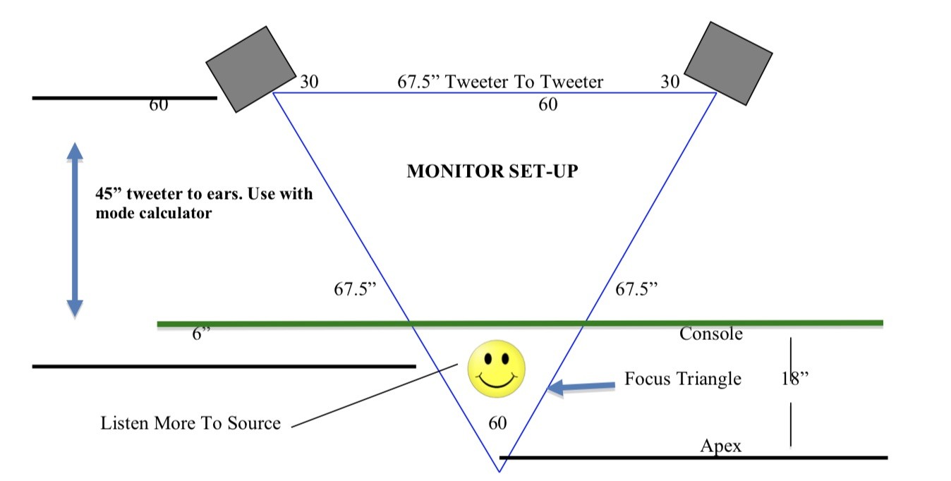
Joining Producer Mike Rodiguez who moderates this webinar for the Audio Engineering Society (AES), Carl focuses this discussion on getting the right sound in audio control rooms. This is done through the ‘Null Positioning Ensemble’ (NPE) which considers the mixing console, listener and the speakers ‘as one’ that can be moved around the room. The ensemble puts the two speakers at about 1.71m apart behind the console firing across the console. Their audio intersects 45cm in front of the console where the listener can sit forming an equilateral triangle. By sitting between the console and where the speakers cross, Carl says you hear the source rather than the speakers thus giving the best audio reproduction.

The NULL POSITIONING ENSEMBLE For Near-Field Monitoring

This effect works if the tweeters are at the same higher as the listener’s ears, says Carl, so should be adjusted to suit the listener. High frequencies are more directional than lower frequencies so for accurate listening, it’s important the speakers aren’t pointing too far off-axis. Exactly where to place your ensemble can seem daunting, but Carl has a calculator on his website which gives a great start allowing you to model your room as a rectangle and find out where the null points are going to be. The nulls are where sound cancels out due to reflections so moving your ensemble to avoid these nulls is the key to a great sound. Carl details how this is done and how, then, to optimise for the ‘real world’ room rather than the mathematical model.

Carl talks about the importance of sound treatment to remove reflections and stop the room from being too lively, with some specific suggestions. In general, the aim is to remove first reflections, have the back stony dead, the ceiling dead and bass traps in the corners. This should allow you to clap your hands without hearing reflection. But you can’t fix every problem with such treatment, Carl says, bringing up a frequency chart of a typical monitor setup which shows a 10dB dip around 125Hz. This is found in all monitoring setups and appears to develop from sound from the speakers bouncing off the floor under the console. He says that this needs to be filled in with subwoofers rather than being fixed with EQ or acoustic treatments.

Watch now!
Speakers

	Carl Tatz Founder, Carl Tatz Design LLC
	Moderator: Mike Rodriguez Freelance Director & Producer

Video: As Time Goes by…Precision Time Protocol in the Emerging Broadcast Networks

Posted on 4th February 2021 by Russell Trafford-Jones

How much timing do you need? PTP can get you timing in the nanoseconds, but is that needed, how can you transport it and how does it work? These questions and more are under the microscope in this video from RTS Thames Valley.

SMPTE Standards Vice President, Bruce Devlin introduces the two main speakers by reminding us why we need timing and how we dealt with it in the past. Looking back to the genesis of television, points out Bruce, everything was analogue and it was almost impossible to delay a signal at all. An 8cm, tightly wound coil of copper would give you only 450 nanoseconds of delay alternatively quartz crystals could be used to create delays. In the analogue world, these delays were used to time signals and since little could be delayed, only small adjustments were necessary. Bruce’s point is that we’ve swapped around now. Delays are everywhere because IP signals need to be buffered at every interface. It’s easy to find buffers that you didn’t know about and even small ones really add up. Whereas analogue TV got us from camera to TV within microseconds, it’s now a struggle to get below two seconds.

Hand in hand with this change is the change from metadata and control data being embedded in the video signal – and hence synchronised with the video signal – to all data being sent separately. This is where PTP, Precision Time Protocol, comes in. An IP-based timing mechanism that can keep time despite the buffers and allow signals to be synchronised.

Next to speak is Richard Hoptroff whose company works with broadcasters and financial services to provide accurate time derived from 4 satellite services (GPS, GLONASS etc) and the Swedish time authority RiSE. They have been working on the problem of delivering time to people who can’t put up antennas either because they are operating in an AWS datacentre or broadcasting from an underground car park. Delivering time by a wired network, Richard points out, is much more practical as it’s not susceptible to jamming and spoofing, unlike GPS.

Richard outlines SMPTE’s ST 2059-2 standard which says that a local system should maintain accuracy to within 1 microsecond. the JT-NM TR1001-1 specification calls for a maximum of 100ms between facilities, however Richard points out that, in practice, 1ms or even 10 microseconds is highly desired. And in tests, he shows that with layer 2, PTP unicast looping around western Europe was able to adhere to 1 microsecond, layer 3 within 10 microseconds. Over the internet, with a VPN Richard says he’s seen around 40 microseconds which would then feed into a boundary clock at the receiving site.

Summing up Richard points out that delivering PTP over a wired network can deliver great timing without needing timing hardware on an OPEX budget. On top of that, you can use it to add resilience to any existing GPS timing.

Gerard Philips from Arista speaks next to explain some of the basics about how PTP works. If you are interested in digging deeper, please check out this talk on PTP from Arista’s Robert Welch.

Already in use by many industries including finance, power and telecoms, PTP is base on IEEE-1588 allowing synchronisation down to 10s of nanoseconds. Just sending out a timestamp to the network would be a problem because jitter is inherent in networks; it’s part and parcel of how switches work. Dealing with the timing variations as smaller packets wait for larger packets to get out of the way is part of the job of PTP.

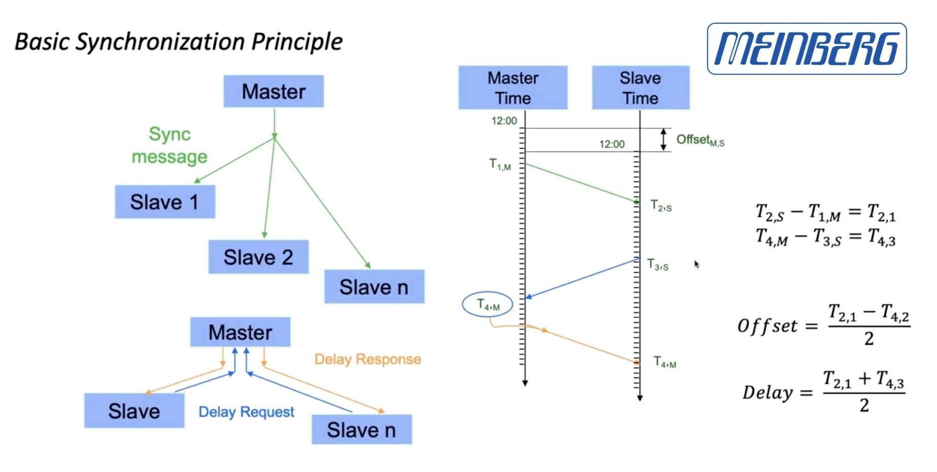
To do this, the main clock – called the grandmaster – sends out the time to everyone 8 times a second. This means that all the devices on the network, known as endpoints, will know what time it was when the message was sent. They still won’t know the actual time because they don’t know how long the message took to get to them. To determine this, each endpoint has to send a message back to the grandmaster. This is called a delay request. All that happens here is that the grandmaster replies with the time it received the message.

PTP Primary-Secondary Message Exchange.
Source: Meinberg [link]

This gives us 4 points in time. The first (t1) is when the grandmaster sent out the first message. The second (t2) is when the device received it. t3 is when the endpoint sent out its delay request and t4 is the time when the master clock received that request. The difference between t2 and t1 indicates how long the original message took to get there. Similarly, t4-t3 gives that information in the other direction. These can be combined to derive the time. For more info either check out Arista’s talk on the topic or this talk from RAVENNA and Meinberg from which the figure above comes.

Gerard briefly gives an overview of Boundary Clock which act as secondary time sources taking pressure off the main grandmaster(s) so they don’t have to deal with thousands of delay requests, but they also solve a problem with jitter of signals being passed through switches as it’s usually the switch itself which is the boundary clock. Alternatively, Transparent Clock switches simply pass on the PTP messages but they update the timestamps to take account of how long the message took to travel through the switch. Gerard recommends only using one type in a single system.

Referring back to Bruce’s opening, Gerard highlights the need to monitor the PTP system. Black and burst timing didn’t need monitoring. As long as the main clock was happy, the DA’s downstream just did their job and on occasion needed replacing. PTP is a system with bidirectional communication and it changes depending on network conditions. Gerard makes a plea to build a monitoring system as part of your solution to provide visibility into how it’s working because as soon as there’s a problem with PTP, there could quickly be major problems. Network switches themselves can provide a lot of telemetry on this showing you delay values and allowing you to see grandmaster changes.

Gerard’s ‘Lessons Learnt’ list features locking down PTP so only a few ports are actually allowed to provide time information to the network, dealing carefully with audio protocols like Dante which need PTP version 1 domains, and making sure all switches are PTP-aware.

The video finishes with Q&A after a quick summary of SMPTE RP 2059-15 which is aiming to standardise telemetry reporting on PTP and associated information. Questions from the audience include asking how easy it is to do inter-continental PTP, whether the internet is prone to asymmetrical paths and how to deal with PTP in the cloud.

Watch now!
Speakers

	Bruce Devlin Standards Vice President, SMPTE
	Gerard Phillips Systems Engineer, Arista
	Richard Hoptroff Founder and CTO Hoptroff London Ltd

Video: PTP in WAN Applications & Update on PTP v2.1

Posted on 1st December 2020 by Russell Trafford-Jones

PTP is evolving as is our ability to use it over WANs. This video explains what’s new in PTP’s second revision and the evolving techniques of using PTP over a wide area network such as the internet. As PTP was built assuming the use of LANs, the longer and more unpredictable latency of WANs throws off the timing calculations, so what can be done to compensate?

In this video from RAVENNA, Andreas Hildebrand from ALC Networx takes us through PTP 2.1, the 2019 revision of PTP following on from PTP 2.0 in 2008 and from the original 1.0 in 2002. Famously, 2.0 and 1.0 were not compatible with each other which has caused problems with some hardware implementations of DANTE which were first written when 1.0 was the only edition. Importantly, Andreas highlights, version 2.1 is backwards compatible with version 2.0. If you’re looking for a PTP primer before digging in, have a look at this intro video from Daniel Boldt, Meinberg

Andreas explains the use of PTP profiles within both AES67 and SMTPTE 2110 which standardise some of the parameters for using PTP such as message frequency. Whilst they do have different defaults, there is an overlap between the two allowing for use of AES67 streams withing both an AES67 ecosystem and with a 2110-30 ecosystem. These overlaps are detailed in the joint AES and SMPTE document, AES-R16-2016.

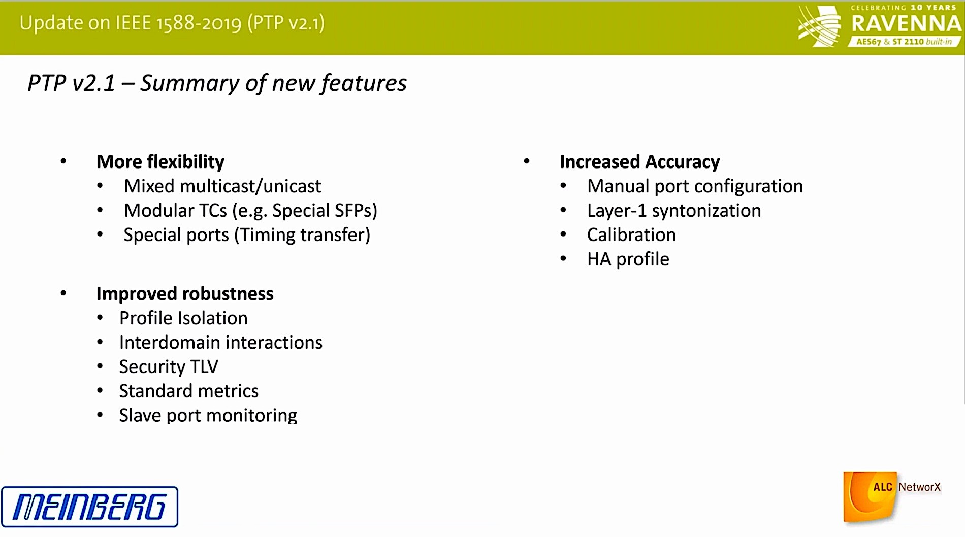
“What’s new in PTP v2.1?” asks Andreas. Apart from clearer language, accuracy, flexibility and robustness have been enhanced.

Flexibility
Flexibility comes from the ability to mixed multicast and unicast messages. Announce and sync messages are still sent in multicast, but queries like delayresponse & delayrequest can now be sent unicast which provides better scalability as, for many scenarios, the reply never needs to go back to any other computers. Another example of flexibility is modular transparent clocks i.e. ones in SFPs. Another flexibility improvement is that it’s now possible to isolate profiles without using different PTP domain numbers. This is by adding a Profile ID called ‘SdoId’.

Robustness and Security
PTP now allows inter-domain interactions effectively allowing multiple GMs to vote onto a single ‘multi-domain clock’. This becomes a very robust clock as it’s created from the insight of three grandmasters. PTP v2.1 adds source integrity checking to allow identification of false, injected, messages. A long-needed improvement as security, even of a LAN, can’t be assumed nowadays.

Performance and Accuracy
Stats reporting has been added to PTP v2.1 allowing monitoring of the average, minimum, max and standard deviation of a number of metrics from the leader clock, delay metrics and message reception counters. Accuracy has been boosted to sub-nanosecond by the CERN-related White Rabbit Project which is an overall benefit to PTP even if sub-nanosecond timing isn’t needed.

Source: ALC NetworX

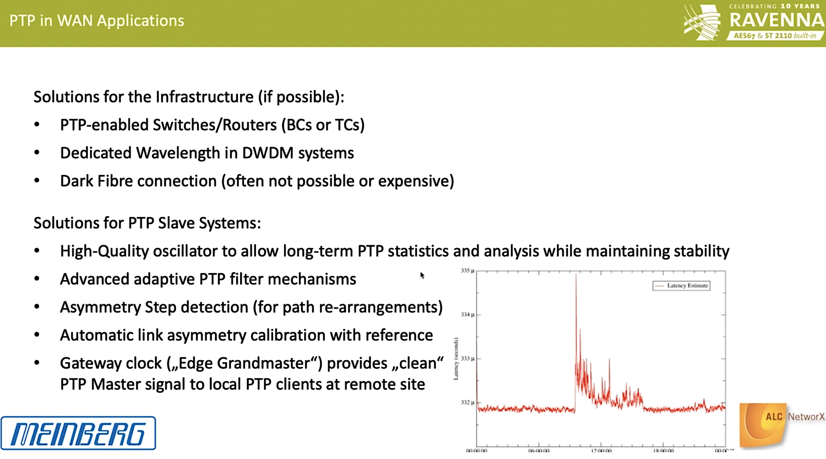
The second part of the video features Meinberg’s Daniel Boldt who discusses how to transmit PTP over the WAN. This is more challenging than a WAN because it’s more likely to be affected by queueing delays – particularly if the WAN in question is the internet. Queueing delays happen for a number of reasons but it all boils down to the fact the switches and routers often have to hold packets in a buffer, something that tends to happen more when there is more load. As such, this means that the delay is variable leading to varying jitter on the measurements.

Another problem often encountered is path changes where a switch happens in the network to divert the signal to a different path. Whilst this is a great way to route around problems, it does mean a sudden change in path length and therefore propagation delay. A conventional ping time may change from 100ms to 250ms in a second. This could have a big impact on the accuracy of a PTP timing signal if undetected.

Finally, the PTP timing algorithm assumes that it takes just as long, and no longer, to get the timing information from A to B as it does to get the follow-up reply from B to A. When one direction takes longer than the other, for instance when one direction is forced through a 100Mbps link rather than 1000Mbps, the PTP timing will have a constant timing error.

Source: Meinberg

Daniel explains that these issues can be mitigated by more thorough processing of the incoming packets. For instance, having a high-quality oscillator which can maintain an accurate frequency for a long time without external input is helpful. Having a local GM on GPS is another good way to avoid problems, in the cases when this is practical, where the WAN PTP becomes an ‘aide’ to timing rather than the authority. Finally, the ‘lucky packets’ technique is demonstrated.

Daniel explains that if you look at the delay of each packet incoming over, say, a two-second period, you can collect all the packets that, based on the timestamp, were lucky enough not to be delayed a lot. By discarding those very-delayed packets, the accuracy of the PTP signal becomes much higher and jitter can reduce, as we see from two case studies, by an order of magnitude.

Watch now!
Speakers