Video: Reliable, Live Contribution over the Internet

For so long we’ve been desperate for a cheap and reliable way to contribute programmes into broadcasters, but it’s only in recent years that using the internet for live-to-air streams has been practical for anyone who cares about staying on-air. Add to that an increasing need to contribute live video into, and out of, cloud workflows, it’s easy to see why there’s so much energy going into making the internet a reliable part of the broadcast chain.

This free on-demand webcast co-produced by The Broadcast Knowledge and SMPTE explores the two popular open technologies for contribution over the internet, RIST and SRT. There are many technologies that pre-date those, including Zixi, Dozer and QVidium’s ARQ to name but 3. However, as the talk covers, it’s only in the last couple of years that the proprietary players have come together with other industry members to work on an open and interoperable way of doing this.

Russell Trafford-Jones, from UK video-over-IP specialist Techex, explores this topic starting from why we need anything more than a bit of forward error correction (FEC) moving on to understanding how these technologies apply to networks other than the internet.

This webcast looks at how SRT and RIST work, their differences and similarities. SRT is a well known protocol created and open sourced by Haivision which predates RIST by a number of years. Haivision have done a remarkable job of explaining to the industry the benefits of using the internet for contibution as well as proving that top-tier broadcasters can rely on it.

RIST is more recent on the scene. A group effort from companies including Haivision, Cobalt, Zixi and AWS elemental to name just a few of the main members, with the aim of making a vendor-agnostic, interoperable protocol. Despite, being only 3 years old, Russell explains the 2 specifications they have already delivered which brings them broadly up to feature parity with SRT and are closing in on 100 members.

Delving into the technical detail, Russell looks at how ARQ, the technology fundamental to all these protocols works, how to navigate firewalls, the benefits of GRE tunnels and much more!

The webcast is free to watch with no registration required.

Watch now!
Speakers

Russell Trafford-Jones Russell Trafford-Jones
Manager, Support & Services, Techex
Director of Education, Emerging Technologies, SMPTE
Editor, The Broadcast Knowledge

Video: Intro into IPv6

It’s certainly taken its time to get here, but IPv6 is increasingly used on the internet. Google now report that just under 30% of the traffic to Google is IPv6 and both Akamai and APNIC show UK IPv6 readiness at around 30% with the US around 50%. Deployment within most enterprise environments, however, is often non existant with many products in the broadcast sector not supporting it at all.

Alex Latzko is an IPv6 evangelist and stands before us to introduce those who are IPv4 savvy to IPv6. For those of us who learnt it once, this is an accessible refresher. Those new to the topic will be able to follow, too, if they have a decent grasp of IPv4. Depending on where you are in the broadcast chain, the impetus to understand IPv6 may be strong, so grab your copy of the slides and let’s watch.

There are no broadcast addresses in IPv6

Alex Latzko
Alex, from ServerCentral Turing Group starts by explaining IPv6 addresses. Familiar to some as a far-too-long mix of hexadecimal numbers and colons, Alex says this is a benefit given the vast range of numbers possible allowing much more flexibility in the way we use the IPv6 address space over IPv4. He takes us through the meanings of the addresses starting with well-known tricks like abbreviating runs of zeros with a double colon, but less well-known ones too, like how to embed IPv4 addresses within an IPv6 address as well as the prefixes for multicast traffic. Alex goes on to show the importance of MAC addresses in IPv6. EUI-64 is a building block used for IPv6 functions which creates a 64-bit string from the 48-bit MAC address. This then allows us to create the important ‘link local’ address.

The last half of the presentation starts with a look at the CIDR prefix lengths that are in use and, is some cases, agreed as standards on the internet at large and in customer networks. For instance, internet routing works on blocks of /48 or larger. Within customer networks, blocks are often /64.

In IPv6, ARP is no longer. ARP can’t work because it uses broadcast addresses which don’t exist within the IPV6 world. This gives rise to the Neighbour Discovery Protocol which allows you to do something very similar. Specifically, it allows you to find your neighbours, routers, detect duplicate addresses and more.

Alex covers whether ‘NAT’ is possible in IPv6 and then looks at how routing works. Starting by imploring us to use ‘proper hierarchy’, he explains that there is no need to conserve IPv6 space. In terms of routing, the landscape is varied in terms of protocols to use. RIP is out of the window, as v1 and v2 have no knowledge of IPv6, OPSFv3 is a beacon of hope, though deployment is often in parallel with the IPv6-ignorant OSPFv2. The good news is that IS-IS, as well as BGP, are perfectly happy with either.

Watch now!
Download the presentation

Speaker

Alex Latzko Alex Latzko
Lead Network Architect
ServerCentral Turing Group

Video: AES67 & SMPTE ST 2110 Timing and Synchronization

Good timing is essential in production for AES67 audio and SMPTE ST 2110. Delivering timing is no longer a matter of delivering a signal throughout your facility, over IP timing is bidirectional and forms a system which should be monitored and managed. Timing distribution has always needed design and architecture, but the detail and understanding needed are much more. At the beginning of this talk, Andreas Hildebrand explains why we need to bother with such complexity, after all, we got along very well for many years without it! Non-IP timing signals are distributed on their own cables as part of their own system. There are some parts of the chain which can get away without timing signals, but when they are needed, they are on a separate cable. With IP, having a separate network for distribution of timing doesn’t make sense so, whether you have an analogue or digital timing signal, that needs to be moving into the IP domain. But how much accuracy in timing to you need? Network devices already widely use NTP which can achieve an accuracy of less than a millisecond. Andreas explains that this isn’t enough for professional audio. At 48Khz, AES samples happen at an accuracy of plus or minus 10 microseconds with 192KHz going down to 2.5 microseconds. As your timing signal has to be less than the accuracy you need, this means we need to achieve nanosecond precision.

Daniel Boldt from timing specialists Meinberg is the focus of this talk explaining how we achieve this nano-second precision. Enter PTP, the Precision Time Protocol. This is a cross-industry standard from the IEEE uses in telcoms, power, finance and in many others wherever a network and its devices need to understand the time. It’s not a static standard, Daniel explains, and it’s just about to see its third revision which, like the last, adds features.

Before finding out about the latest changes, Daniel explains how PTP works in the first place; how is it possible to accurately derive time down to the nanosecond over a network which will have variable propagation times? We see how timestamps are introduced into the network interface controller (NIC) at the last moment allowing the timestamps to be created in hardware which removes some of the variable delays that is typical in software. This happens, Daniel shows, in the switch as well as in the server network cards. This article will refer to either a primary clock or a grand master. Daniel steps us through the messages exchanged between the primary and secondary clock which is the interaction at the heart of the protocol. The key is that after the primary has sent a timestamp, the secondary sends its timestamp to the primary which replies saying the time it received the secondary the reply. The secondary ends up with 4 timestamps that it can combine to determine its offset from the primary’s time and the delay in receiving messages. Applying this information allows it to correct the clock very accurately.

PTP Primary-Secondary Message Exchange.
Source: Meinberg

Most broadcasters would prefer to have more than one grandmaster clock but if there are multiple clocks, how do you choose which to sync from? Timing systems have long used strata whereby clocks are rated based on accuracy, either for internal accuracy & stability or by what they are synched to. This is also true for PTP and is part of the considerations in the ‘Best Master Clock Algorithm’. The BMCA starts by allowing a time source to assess its own accuracy and then search for better options on the network. Clocks announce themselves to the network and by listening to other announcements, a clock can decide if it should become a primary clock if, for instance, it hears no announce messages at all. For devices which should never be a grand primary, you can force them never to decide to become grand masters. This is a requisite for audio devices participating in ST 2110-3x.

Passing PTP around the network takes some care and is most easily done by using switches which understand PTP. These switches either run a ‘boundary clock’ or are ‘transparent clocks’. Daniel explores both of these scenarios explaining how the boundary clock switch is able to run multiple primary and secondary clocks depending on what is connected on each interface. We also see what work the switches have to do behind the scenes to maintain timing precision in transparent mode. In summary, Daniel summaries boundary clocks as being good for hierarchical systems and scales well but requires continuous monitoring whereas transparent clocks are simpler to deploy and require minimal monitoring. The main issue with transparent clocks is that they don’t scale well as all your timing messages are still going back to one main clock which could get overwhelmed.

SMPTE 2022-7 has been a very successful standard as its reliance only on RTP has allowed it to be widely applicable to compressed and uncompressed IP flows. It is often used in 2110 networks, too, where two separate networks are run and brought together at the receiving device. That device, on a packet-by-packet basis, is free to derive its audio/video stream from either network. This requires, however, exactly the same timing on both networks so Daniel looks at an example diagram where this PTP sharing is shown.

PTP’s still evolving and in this next section, Daniel takes us through some of the coming improvements which are also outlined at Meinberg’s blog. These are profile isolation, multi-domain clocks, security improvements and more.

Andreas takes the final section of the webinar to explain how we use PTP in media networks. All receivers will have the same clock which could be derived from GPS removing the need to distribute PTP between sites. 2110 is based on RTP which requires a timestamp to be added to every packet delivered to the network. RTP is a wrapper around IP packets which includes a timestamp which can be derived from the media clock counter.

Andreas looks at how accurate RTP delivery is achieved, dealing with offset values, populating the timestamp from the PTP clock for realties streams and he explains how the playout delay is calculated from the link offset. Finally, he shows the relatively simple process of synchronisation art the playout device. With all the timestamps in the system, synchronising playback of audio, video and metadata using buffers can be achieved fairly easily. Unfortunately, timestamps are easily destroyed by secondary processing (for instance loudness adjustment for an audio stream). Clearly, if this happened, synchronisation at the receiver would be broken. Whilst this will be addressed by out-of-band messaging in future standards, for now, this is managed by a broadcast controller which can take delay information from processing stages and distribute this to receivers.

Watch now!
Speakers

Daniel Boldt Daniel Boldt
Head of Software Development,
Meinberg
Andreas Hildebrand Andreas Hildebrand
RAVENNA Technology Evangelist,
ALC NetworX

Video: Colour Theory

Understanding the way colour is recorded and processed in the broadcast chain is vital to ensuring its safe passage. Whilst there are plenty of people who work in part of the broadcast chain which shouldn’t touch colour, being purely there for transport, the reality is that if you don’t know how colour is dealt with under the hood, it’s not possible to any technical validation of the signal beyond ‘it looks alright!’. The problem being, if you don’t know what’s involved in displaying it correctly, or how it’s transported, how can you tell?

Ollie Kenchington has dropped into the CPV Common Room for this tutorial on colour which starts at the very basics and works up to four case studies at the end. He starts off by simply talking about how colours mix together. Ollie explains the difference between the world of paints, where mixing together is an act of subtracting colours and the world of mixing light which is about adding colours together. Whilst this might seem pedantic, it creates profound differences regarding what colour two mixed colours create. Pigments such as paints look that way because they only reflect the colour(s) you see. They simply don’t reflect the other colours. This is why they are called subtractive; shine a blue light on something that is pure red, and you will just see black, because there is no red light to reflect back. Lights, however, provide lights and look that way because they are sending out the light you see. So mixing a red and blue light will create magenta. This is known as additive colour mixing and introduces color.adobe.com which lets you discover new colour palettes.

The colour wheel is next on the agenda which Ollie explains allows you to talk about the amplitude of a colour – the distance the colour is from the centre of the circle – and the angle that defines the colour itself. But as important as it is to describe a colour in a document, it’s all the more important to understand how humans see colours. Ollie lays out the way that rods & cones work in the eye. That there is a central area that sees the best detail and has most of the cones. The cones, we see, are the cells that help us see colour. The fact there aren’t many cones in our periphery is covered up by our brains which interpolate colour from what they have seen and what they know about our current environment. Everyone is colour blind, Ollie explains, in our peripheral vision but the brain makes up for it all from what it knows about what you have seen. Overall, in your eye, sensitivity to blue is by far much less than that you have for green and then red. This is because, in evolutionary terms, there is much less important information gained by seeing detail in blue than in green, the colour of plants. Red, of course, helps understanding shades of green and brown which are both colours native to plants. The upshot of this, Ollie explains, is that when we come to processing light, we have to do it in a way that takes into account the human sensitivity to different wavelengths. This means that we can show three rectangles next to each other, red, green and blue, see them as similar brightnesses but then see that under the hood, we’ve reduced the intensity of the blue by 89 per cent, the red by 70 and the green by only 41. When added together, these show the correct greyscale brightness.

The CIE 1931 colour space is the next topic. The CIE 1931 colourspace shows all the colours that the human eye can see. Ollie demonstrates, by overlaying it on the graph that ITU-R Rec.709 – broadcast’s most well-known and most widely-used colourspace only provides 35% coverage of what our eyes can see. This makes the call for Rec 2020 from the proponents of UHD and ‘better pixels’, which covers 75%, all the more relevant.

Ollie next focuses in on acquisition talking about CMOS chips in cameras which are monochromatic by nature. As each pixel of a CMOS sensor only records how many photons it received, it is intrinsically monochrome. Therefore, in order to show colour, you need to put a Bayer colour filter array in front. Essentially this describes a pattern of red, blue and green filters above this pixel. With the filter in place, you know that the value you read from a given pixel represents just that single colour. If you put red, blue and green filters over a range of pixels on the sensor, you are able to reconstruct the colour of the incoming scene.

Ollie then starts to talk about reducing colour date. We an do this at source by only recording 8, rather than 10-bits of colour, but Ollie shows us a clear demonstration of when that doesn’t look good; typically 8-bit video lets itself down on sunsets, flesh tones or similar subtle. gradients. The same principle drives the HDR discussion regarding 10-bit Vs. 12 bit. With PQ being built for 12-bit, but realistic live production workflows for the next few years being 10-bit which HLG expects, there is plenty of water to go under the bridge before we see whether PQ’s 12-bit advantage really comes into its own outside of cinemas. Ollie also explains colour subsampling which gets a thorough explanation detailing not only 4:4:4 and 4:2:2 but also the less common examples.

The next section looks at ‘scopes’ also known as ‘waveform monitors’. Ollie starts with the histogram which shows you how much of your picture is a certain brightness helping understanding how exposed your picture is overall. With the histogram, the horizontal axis shows brightness with the left being black and the right being white. Whereas the waveform shows the brightness on the horizontal and then the x axis shows you the position in the picture that a certain brightness happens. This allows you to directly associate brightness values with objects in the scene. This can be done with the luma signal or the separate RGB which then allows you to understand the colour of that area. Vectorscope

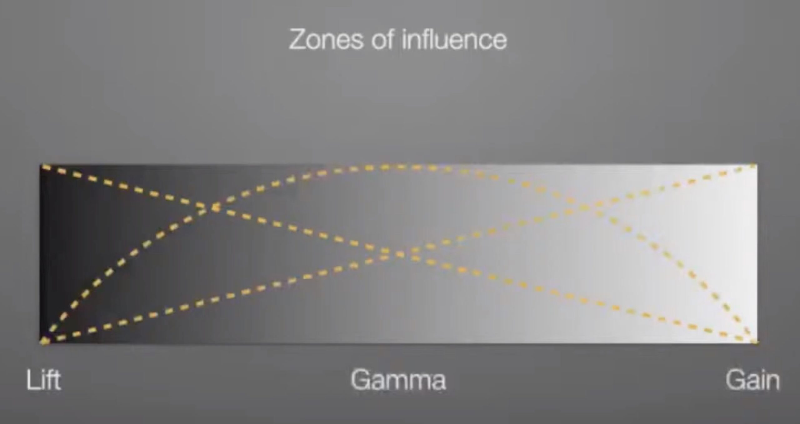
Ollie then moves on to discussing balancing contrast looking at lift (lifting the black point), gamma (affects central), gain (altering the white point) and mixing that with shadows, midtones and highlights. He then talks about how the surroundings affect your perceived brightness of the picture and shows it with great boxes in different surrounds. Ollie demonstrates this as part of the slides in the presentation very effectively and talks about the need for standards to control this. When grading, he discusses the different gamma that screens should be set to for different types of work and discusses the standard which says that the ambient light in the surrounding room should be about 10% as bright as the screen displaying pure white.

The last part of the talk presents case studies of programmes and films looking at the way they used colour, saturation, costume and lighting to enhance and underwrite the story that was being told. This takeaway is the need to think of colour as a narrative element. Something that can be informed from and understood by wardrobe, visual look intention, wardrobe and lighting. The conversation about colour and grading should start early in the filming process and a key point Ollie makes is that this is not a conversation that costs a lot, but having it early in the production is priceless in terms of its impact on the cost and results of the project.

Watch now!
Speakers

Ollie Kenchington Ollie Kenchington
Owner & Creative Director,
Korro Films, Korro Academy